Ridgeline Plot

::code-group

# %%
import numpy as np
import matplotlib.pyplot as plt
import pandas as pd
from scipy.stats import gaussian_kde

from src.config import DATA_PATH

# %%
# Years to include
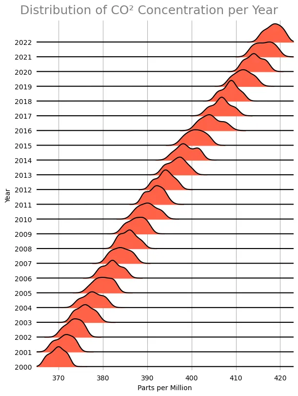
YEAR_RANGE = (2000, 2022)
# X-axis resolution
N_POINTS = 200
# Overlap in the ridgeline plot
OVERLAP = 0.85

# %%
# Read data from file
data = pd.read_csv(DATA_PATH / "co2-trends.csv")
# Limit data to between the specified years and columns to year and ppm. Also drop missing.
co2 = data.loc[lambda x: x["year"].between(*YEAR_RANGE), ["year", "ppm"]].dropna()

# %%
years = np.arange(YEAR_RANGE[0], YEAR_RANGE[1] + 1)
y_baseline = np.arange(len(years)) * (1 - OVERLAP)

x = np.linspace(365, 423, N_POINTS)

densities = np.stack(
    co2.groupby("year").apply(lambda d: gaussian_kde(d["ppm"])(x)).values
)

ys = (y_baseline + densities.T).T

# %%
fig, ax = plt.subplots(figsize=(6, 8), constrained_layout=True)

for b, y in zip(y_baseline, ys):
    plt.fill_between(
        x, np.ones(N_POINTS) * b, y, where=~np.isclose(b, y), color="tomato"
    )
    plt.plot(x, y, c="black")

ax.set_yticks(y_baseline)
ax.set_yticklabels(years)

ax.set_xlabel("Parts per Million")
ax.set_ylabel("Year")

ax.margins(x=0, y=0.01)
ax.tick_params(axis="both", bottom=False, left=False)
ax.set_axisbelow(True)

ax.grid(True, axis="x")

ax.spines["top"].set_visible(False)
ax.spines["right"].set_visible(False)
ax.spines["bottom"].set_visible(False)
ax.spines["left"].set_visible(False)

fig.suptitle("Distribution of CO² Concentration per Year", fontsize=18, color="gray")

::code-block{label="Result"}

![Ridgeline Plot](@assets/img/examples/ridgeline-plot.png)

:: ::